7.4. Working with cycles#
This section introduces the ktk.cycles module and its functions:
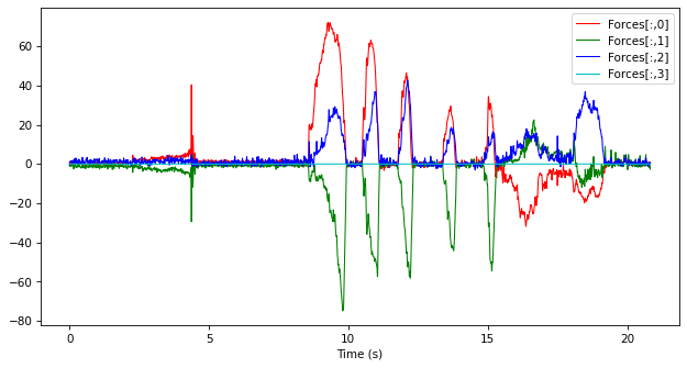
For this section, we will use a dataset of wheelchair propulsion kinetics.
import kineticstoolkit.lab as ktk
import pandas as pd
import numpy as np
import matplotlib.pyplot as plt

filename = ktk.doc.download("kinetics_wheelchair_propulsion.ktk.zip")
ts = ktk.load(filename)

ts.plot("Forces")
7.4.1. Detecting cycles#
Warning
This section may change by the time Kinetics Toolkit reaches version 1.0. The current function ktk.cycles.detect_cycles attempts to do too much and therefore it is not generic enough. In the future, it will likely be replaced by several, more specific and more optimized functions. It will however likely stay available for several years, as it is not deprecated yet, and deprecated functions live for 2 years before removal.
The ktk.cycles.detect_cycles function detects biphasic cycles in a TimeSeries, and adds transitions as events. Each cycle has three events:
The start of the first phase, named using the
event_namesparameters;The start of the second phase, also named using the
event_namesparameters;The end of the cycle, always named
_.
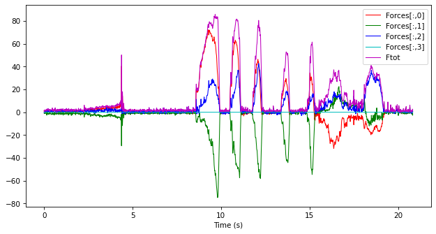
The function does not modify the TimeSeries data, only the events. It uses two thresholds applied to a unidimensional signal from the TimeSeries. In this example, this signal will be the total force \(F_{tot}\). This could also apply to gait, or one could also use only the vertical ground reaction force, depending on the lab’s conventions or methods.
Let’s calculate \(F_{tot}\) based on the three force components, and add it as a new data of the TimeSeries as it will be our source for detecting the cycles.
ts = ts.add_data(
    "Ftot", np.sqrt(np.sum(ts.data["Forces"] ** 2, axis=1))
)

ts.plot(["Forces", "Ftot"])
We then define some threshold values for \(F_\text{tot}\):
Push starts when \(F_\text{tot}\) raises to more than 10 N;
Recovery starts when \(F_\text{tot}\) decreases to less than 5 N.
ts_with_events = ktk.cycles.detect_cycles(
    ts, "Ftot", event_names=["push", "recovery"], thresholds=[10, 5]
)
ts_with_events.plot(["Forces", "Ftot"])

We observe that most cycles are well identified, but more cycles have been identified. We can reject “false” cycles based on a minimal duration:
ts_with_events = ktk.cycles.detect_cycles(
    ts,
    "Ftot",
    event_names=["push", "recovery"],
    thresholds=[10, 5],
    min_durations=[0.2, 0.2],
)
ts_with_events.plot(["Forces", "Ftot"])
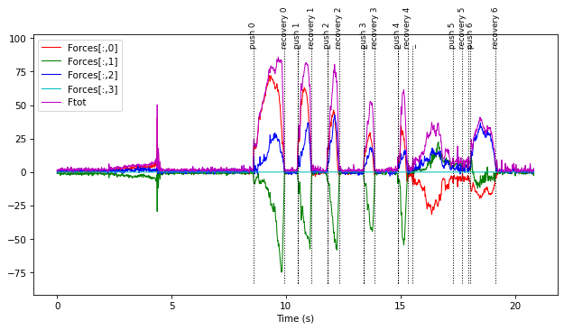
There are other arguments available to filter out more cycles, such as max durations, and minimal/maximal peak height. These arguments are documented in the ktk.cycles.detect_cycles function. Here, we may reject pushes that do not reach a minimal peak height of 45 N.
ts_with_events = ktk.cycles.detect_cycles(
    ts,
    "Ftot",
    event_names=["push", "recovery"],
    thresholds=[10, 5],
    min_durations=[0.2, 0.2],
    min_peak_heights=[45, -np.Inf],
)
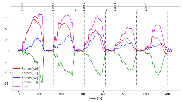
ts_with_events.plot(["Forces", "Ftot"])
plt.tight_layout()

Tip
We observe an _ event at the end. There are in fact such _ events at the end of each cycle (look how each next push’s ‘p’ letter seems underlined). As explained above, the detect_cycles function adds an _ event at the end of each cycle. These events are usefull to extract cycles of phases using TimeSeries methods such as ktk.TimeSeries.get_ts_between_events.
Good practice: Manual editing
Although detecting cycles automatically seems time-saving, it is always an excellent idea to manually inspect any signal that is being processed based on such “arbitrary” constraints. Use the interactive ktk.TimeSeries.ui_edit_events method to inspect, correct and manually identify cycles.
7.4.2. Time-normalizing cycles#
Once the cycles have been detected, we can time-normalize them using ktk.cycles.time_normalize. Here, every complete cycle will be time-normalized from 0 to 100%.
ts_normalized_on_cycle = ktk.cycles.time_normalize(
    ts_with_events, event_name1="push", event_name2="_"
)

ts_normalized_on_cycle.plot(["Forces", "Ftot"])

To time-normalize only during the push phase, we would define event_name2 as “recovery” instead of “ _ “:
ts_normalized_on_push = ktk.cycles.time_normalize(
    ts_with_events, "push", "recovery"
)

ts_normalized_on_push.plot(["Forces", "Ftot"])
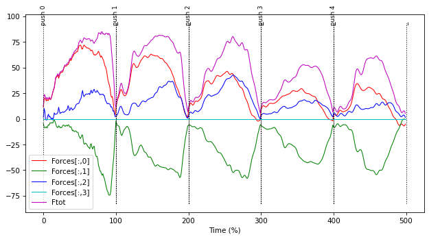
It is also possible to include data before 0% and after 100% using the span parameter. For example, to include pre-push (-25% to 0%) and post-recovery (100% to 125%):
ts_normalized_on_push_with_span = ktk.cycles.time_normalize(
    ts_with_events, "push", "recovery", span=[-20, 125]
)

ts_normalized_on_push_with_span.plot(["Forces", "Ftot"])
In this case, each time point still represents 1% of a cycle, but the TimeSeries wrap every 145 points (0 to 19 is the pre-push for the first cycle, 20 to 119 is the first push, 120 to 144 is the post-release for the first cycle, etc.).
7.4.3. Combining the cycles#
Cycles are often analyzed together. The ktk.cycles.stack generates a dictionary of numpy arrays with the first dimension being the cycle and the second being the percentage of cycle.
data = ktk.cycles.stack(ts_normalized_on_push)

data
{
     'Forces': <array of shape (5, 100, 4)>
    'Moments': <array of shape (5, 100, 4)>
       'Ftot': <array of shape (5, 100)>
}
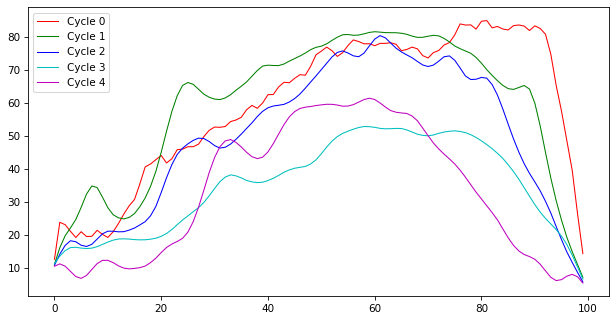
It is now easier to perform operations on ensembles of cycles. For example, to plot \(F_\text{tot}\) in each cycle one of top of the other:
n_cycles = data["Ftot"].shape[0]
for i_cycle in range(n_cycles):
    plt.plot(data["Ftot"][i_cycle], label=f"Cycle {i_cycle}")

plt.legend();
The inverse operation of ktk.cycles.stack is ktk.cycles.unstack.
7.4.4. Finding the most repeatable cycles#
We can sort the cycles in order of reproducibility (get which cycles are the most repeatable, and which cycles are unique) using ktk.cycles.most_repeatable_cycles. Here, we will base this analysis on the Ftot signal.
index = ktk.cycles.most_repeatable_cycles(data["Ftot"])

index
[1, 2, 0, 3, 4]
We see that cycles 1 and 2 were identified to be the most representative of all cycles, while cycles 3 and 4 are the most different. However, please keep in mind that this operation is not optimal for so few cycles (five total).
