10.5. Styling and exporting

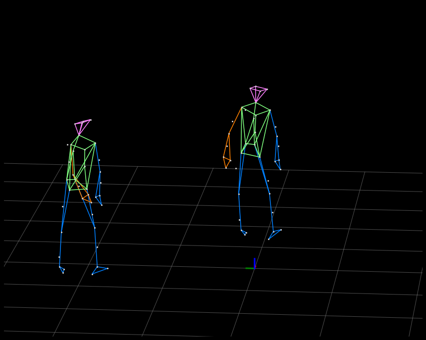
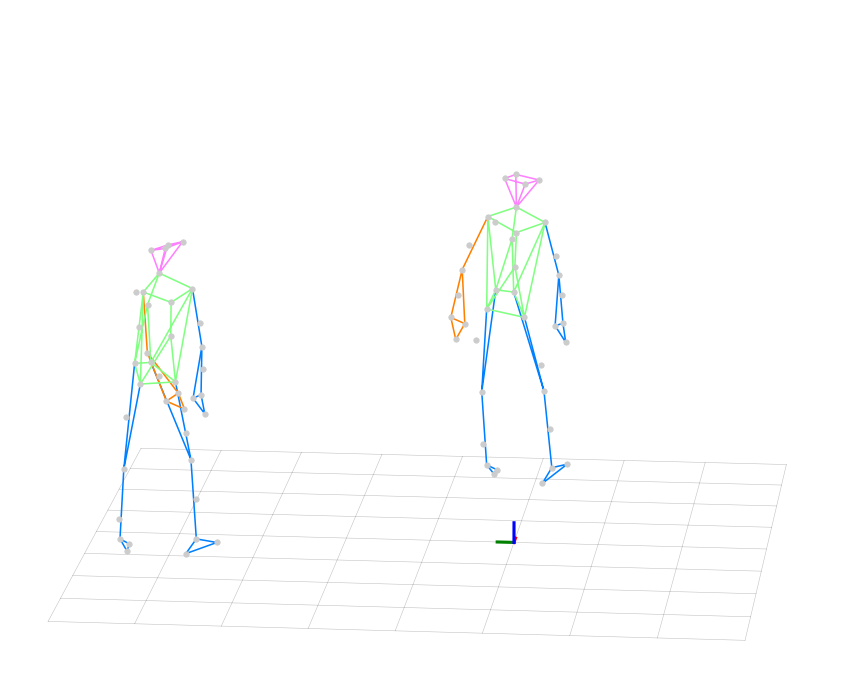
Every element of the Player can be stylized. Let’s load the tennis serve data again, then we will use the properties of the Player to style its elements.

Show code cell content Hide code cell content

import kineticstoolkit.lab as ktk

# Download and read markers from a sample C3D file
filename = ktk.doc.download("kinematics_tennis_serve_2players.c3d")
markers = ktk.read_c3d(filename)["Points"]
interconnections = dict()  # Will contain all segment definitions
interconnections["LLowerLimb"] = {
    "Color": (0, 0.5, 1),  # In RGB format (here, greenish blue)
    "Links": [  # List of lines that span lists of markers
        ["*LTOE", "*LHEE", "*LANK", "*LTOE"],
        ["*LANK", "*LKNE", "*LASI"],
        ["*LKNE", "*LPSI"],
    ],
}
interconnections["RLowerLimb"] = {
    "Color": (0, 0.5, 1),
    "Links": [
        ["*RTOE", "*RHEE", "*RANK", "*RTOE"],
        ["*RANK", "*RKNE", "*RASI"],
        ["*RKNE", "*RPSI"],
    ],
}
interconnections["LUpperLimb"] = {
    "Color": (0, 0.5, 1),
    "Links": [
        ["*LSHO", "*LELB", "*LWRA", "*LFIN"],
        ["*LELB", "*LWRB", "*LFIN"],
        ["*LWRA", "*LWRB"],
    ],
}
interconnections["RUpperLimb"] = {
    "Color": (1, 0.5, 0),
    "Links": [
        ["*RSHO", "*RELB", "*RWRA", "*RFIN"],
        ["*RELB", "*RWRB", "*RFIN"],
        ["*RWRA", "*RWRB"],
    ],
}
interconnections["Head"] = {
    "Color": (1, 0.5, 1),
    "Links": [
        ["*C7", "*LFHD", "*RFHD", "*C7"],
        ["*C7", "*LBHD", "*RBHD", "*C7"],
        ["*LBHD", "*LFHD"],
        ["*RBHD", "*RFHD"],
    ],
}
interconnections["TrunkPelvis"] = {
    "Color": (0.5, 1, 0.5),
    "Links": [
        ["*LASI", "*STRN", "*RASI"],
        ["*STRN", "*CLAV"],
        ["*LPSI", "*T10", "*RPSI"],
        ["*T10", "*C7"],
        ["*LASI", "*LSHO", "*LPSI"],
        ["*RASI", "*RSHO", "*RPSI"],
        ["*LPSI", "*LASI", "*RASI", "*RPSI", "*LPSI"],
        ["*LSHO", "*CLAV", "*RSHO", "*C7", "*LSHO"],
    ],
}
p = ktk.Player(
    markers,
    interconnections=interconnections,
    up="z",
    anterior="-y",
    target=(0, 0.5, 1),
    azimuth=0.1,
    zoom=1.5, 
)

10.5.1. Styling the background

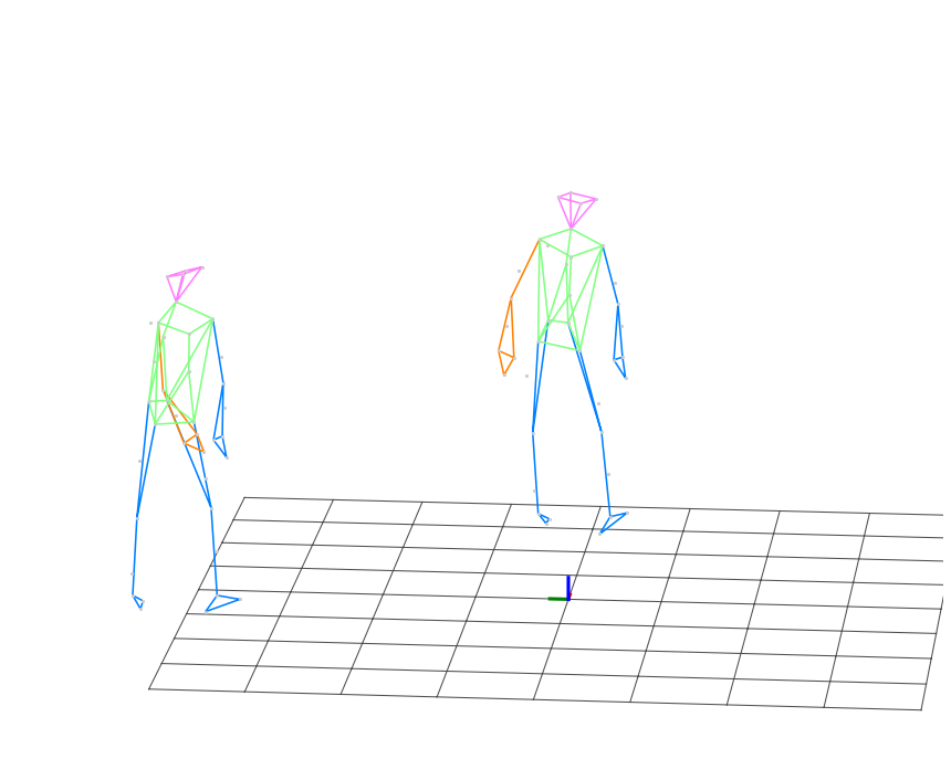
To set a white background:

p.background_color = 'w'

# Equivalent to p.background_color = (1.0, 1.0, 1.0)

10.5.2. Styling the grid

10.5.2.1. Grid size and subdivisions

To have a smaller grid (4x4 metres) with a smaller subdivision size (50x50 cm):

p.grid_size = 4
p.grid_subdivision_size = 0.5

10.5.2.2. Grid origin

The grid origin can be placed anywhere in the scene, using the grid_origin property. For example:

p.grid_origin = (0.0, 0.5, 0.0)

10.5.2.3. Grid width

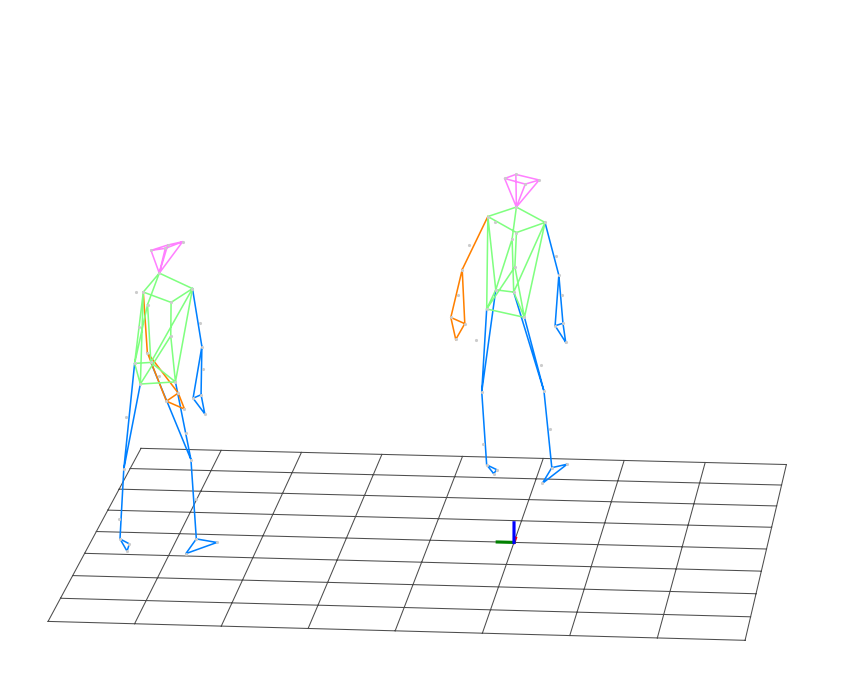
To get a thinner grid:

p.grid_width = 0.5

10.5.2.4. Grid colour

To get a light grey grid:

p.grid_color = (0.75, 0.75, 0.75)

10.5.3. Styling points

10.5.3.1. Point size

To get bigger points:

p.point_size = 10

10.5.3.2. Point colour

The default point colour can be set by the default_point_color property:

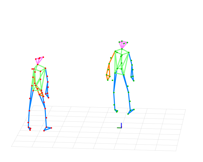
p.default_point_color = 'r'

# Equivalent to: p.default_point_color = (1.0, 0.0, 0.0)

To assign individual colours, we add a Color info to the TimeSeries’ data. For instance, to show Viktor’s markers in dark green:

markers = p.get_contents()

for key in markers.data:
    if key.startswith("Viktor:"):
        markers = markers.add_data_info(key, "Color", (0.0, 0.75, 0.0))

p.set_contents(markers)

10.5.4. Styling interconnections

10.5.4.1. Interconnection width

To get thicker interconnections:

p.interconnection_width = 4.0

10.5.4.2. Interconnection colour

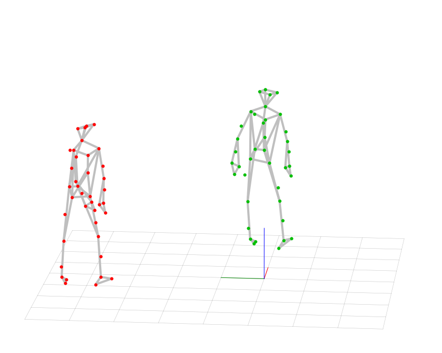
Colour is part of the interconnection dictionary. Therefore, we change interconnection colour using this dictionary. For instance, to set all interconnections to light grey:

interconnections = p.get_interconnections()

for segment in interconnections:
    interconnections[segment]["Color"] = (0.75, 0.75, 0.75)

p.set_interconnections(interconnections)

10.5.5. Styling frames

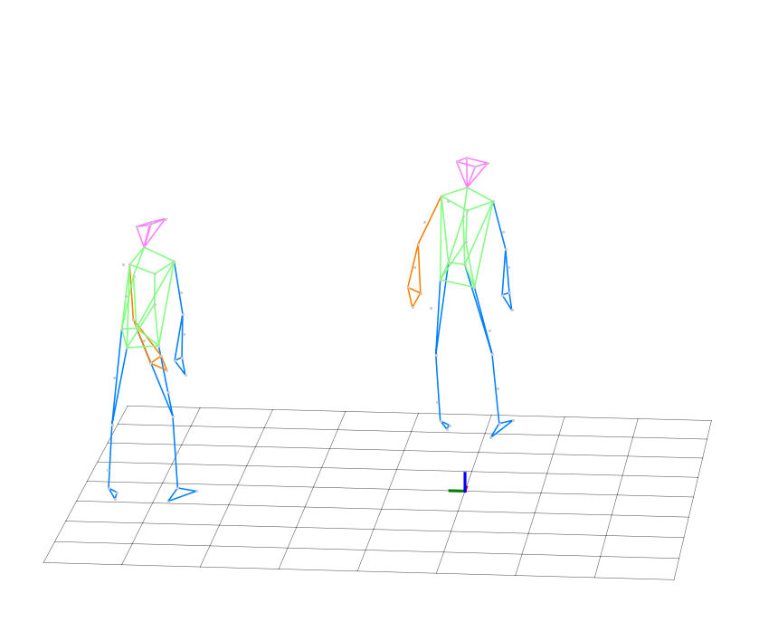
10.5.5.1. Frame size

To get half-metre long frames:

p.frame_size = 0.5

10.5.5.2. Frame width

To get thinner frames:

p.frame_width = 1.0

10.5.6. Exporting

10.5.6.1. Exporting to an image

The Player’s current view can be exported to any file format supported by Matplotlib such as PNG, JPEG, SVG, or PDF, using ktk.Player.to_image:

p.to_image("exported_image.png")

10.5.6.2. Exporting to a video

The whole animation in the current viewpoint can be exported to an MP4 file using ktk.Player.to_video:

p.to_video("exported_video.mp4")

Note

To create videos, the package ffmpeg must be installed on your computer. If you installed Kinetics Toolkit using conda, then it is already installed. If you used pip, you must install it manually.