5.11.2. Exercise: Indexing/slicing/filtering one-dimensional arrays 2#
The position of an object was recorded in meters over one second at a sampling frequency of 100 Hz:
import numpy as np

p = np.array(
    [
        0.    , 0.0099, 0.0196, 0.0291, 0.0384, 0.0475, 0.0564, 0.0651,
        0.0736, 0.0819, 0.09  , 0.0979, 0.1056, 0.1131, 0.1204, 0.1275,
        0.1344, 0.1411, 0.1476, 0.1539, 0.16  , 0.1659, 0.1716, 0.1771,
        0.1824, 0.1875, 0.1924, 0.1971, 0.2016, 0.2059, 0.21  , 0.2139,
        0.2176, 0.2211, 0.2244, 0.2275, 0.2304, 0.2331, 0.2356, 0.2379,
        0.24  , 0.2419, 0.2436, 0.2451, 0.2464, 0.2475, 0.2484, 0.2491,
        0.2496, 0.2499, 0.25  , 0.2499, 0.2496, 0.2491, 0.2484, 0.2475,
        0.2464, 0.2451, 0.2436, 0.2419, 0.24  , 0.2379, 0.2356, 0.2331,
        0.2304, 0.2275, 0.2244, 0.2211, 0.2176, 0.2139, 0.21  , 0.2059,
        0.2016, 0.1971, 0.1924, 0.1875, 0.1824, 0.1771, 0.1716, 0.1659,
        0.16  , 0.1539, 0.1476, 0.1411, 0.1344, 0.1275, 0.1204, 0.1131,
        0.1056, 0.0979, 0.09  , 0.0819, 0.0736, 0.0651, 0.0564, 0.0475,
        0.0384, 0.0291, 0.0196, 0.0099
    ]
)
Knowing that:
\[
v(i) = \dfrac{p(i+1) - p(i-1)}{t(i+1) - t(i-1)}
\]
Write a program of only 1 to 2 lines that calculates the speed of the object. Then, plot the velocity and position on the same figure to check your result.
Tip
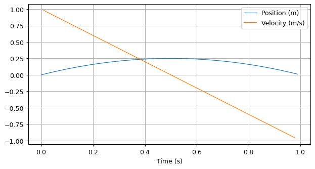
Due to the calculation of speed requiring position values before and after the current sample, the velocity array will be 2 values shorter than the position array, as illustrated in Fig. 5.9.

Fig. 5.9 Calculating speed leads to a shorter array.#
Show code cell content
import numpy as np
import matplotlib.pyplot as plt

t = np.arange(100) / 100
v = (p[2:] - p[0:-2]) / (t[2:] - t[0:-2])

# Since the time step is regular at 0.01, we could also calculate v using a single line:
v = (p[2:] - p[0:-2]) / (2 * 0.01)

# Plot the result
plt.plot(t, p, label="Position (m)")
plt.plot(t[1:-1], v, label="Velocity (m/s)")
plt.xlabel("Time (s)")
plt.grid(True)
plt.legend()
plt.show()