7.2.3. Time management

This section shows how to use these methods for time management:

• ktk.TimeSeries.get_sample_rate

• ktk.TimeSeries.resample

• ktk.TimeSeries.shift

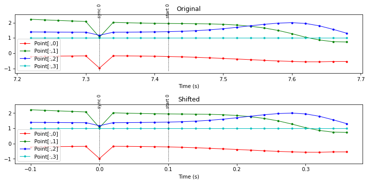
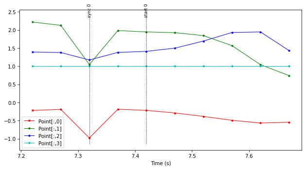
We will use this sample TimeSeries:

import kineticstoolkit.lab as ktk
import numpy as np
import matplotlib.pyplot as plt

ts = ktk.TimeSeries()
ts.time = np.arange(722, 770, 2) / 100
ts = ts.add_data(
    "Point",
    np.array(
        [
            [-0.21952191, 2.21998239, 1.3917855, 1.0],
            [-0.20554896, 2.18186331, 1.3860414, 1.0],
            [-0.19351672, 2.14477563, 1.38044441, 1.0],
            [-0.18593165, 2.11034703, 1.37598848, 1.0],
            [-0.17999941, 2.07810235, 1.37413812, 1.0],
            [-0.97747644, 1.04681897, 1.17331319, 1.0],
            [-0.1770632, 2.01822352, 1.37383687, 1.0],
            [-0.18178312, 1.99475348, 1.37715793, 1.0],
            [-0.18880549, 1.97409928, 1.3846097, 1.0],
            [-0.20046318, 1.95866096, 1.39489722, 1.0],
            [-0.21780199, 1.94720566, 1.4106667, 1.0],
            [-0.24116059, 1.93896806, 1.43488669, 1.0],
            [-0.27086243, 1.93140829, 1.47220325, 1.0],
            [-0.30681622, 1.91995525, 1.52735615, 1.0],
            [-0.34540462, 1.89304924, 1.60226464, 1.0],
            [-0.3847855, 1.84441411, 1.69457984, 1.0],
            [-0.42655963, 1.76527178, 1.79648793, 1.0],
            [-0.47107416, 1.64915574, 1.89288461, 1.0],
            [-0.51133025, 1.49018431, 1.96876347, 1.0],
            [-0.54127008, 1.28111708, 2.00170565, 1.0],
            [-0.56586808, 1.04348814, 1.9465847, 1.0],
            [-0.5676325, 0.86329579, 1.79276991, 1.0],
            [-0.5448004, 0.75350696, 1.56222212, 1.0],
            [-0.54447311, 0.73373014, 1.30583119, 1.0],
        ]
    )
)
ts = ts.add_event(7.32, "sync")
ts = ts.add_event(7.42, "start")

ts.plot([], ".-")

7.2.3.1. Sample rate

To know the sample rate of a TimeSeries (i.e., the number of data points per second), we use ktk.TimeSeries.get_sample_rate:

ts.get_sample_rate()

50.00000000000001

7.2.3.2. Resampling

To resample the TimeSeries to a different sample rate, we use ktk.TimeSeries.resample, which takes either a new frequency or a new time array as an argument. To downsample our TimeSeries to 20Hz, we would do:

ts_20Hz = ts.resample(20.0)

which gives:

Good practice: Filtering before downsampling

It is usually important to filter a signal before downsampling it, to respect the Nyquist–Shannon sampling theorem and thus avoid aliasing.

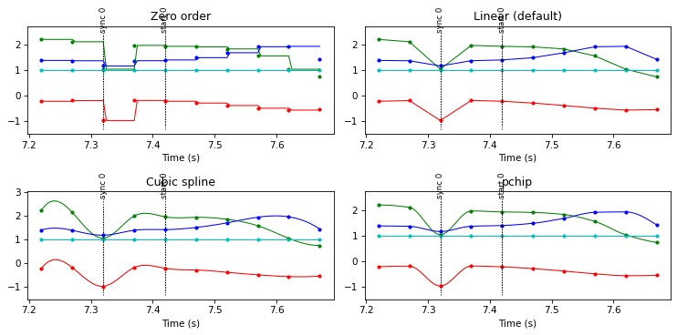
We use the same method to upsample a signal. Note that in this case, we may want to select the interpolation method since different interpolation methods may produce much different results. For example, if we upscale the ts_20Hz signal using different interpolation methods:

# Zero order (sample-and-hold)
ts_200Hz_zero = ts_20Hz.resample(200.0, kind="zero")

# Linear (default)
ts_200Hz_linear = ts_20Hz.resample(200.0, kind="linear")

# Cubic spline
ts_200Hz_cubic = ts_20Hz.resample(200.0, kind="cubic")

# Piecewise Cubic Hermite Interpolating Polynomial (pchip)
ts_200Hz_pchip = ts_20Hz.resample(200.0, kind="pchip")

we get:

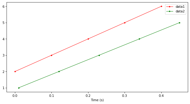
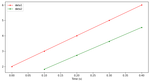
Instead of specifying a new frequency, we can resample directly to a new time array. This is practical to combine data from individual instruments that may have their own sampling frequency.

instrument1 = ktk.TimeSeries()
instrument2 = ktk.TimeSeries()

instrument1.time = np.array([0.0, 0.1, 0.2, 0.3, 0.4])
instrument2.time = np.array([0.01, 0.12, 0.23, 0.34, 0.45])

instrument1.data['data1'] = np.array([2.0, 3.0, 4.0, 5.0, 6.0])
instrument2.data['data2'] = np.array([1.0, 2.0, 3.0, 4.0, 5.0])

instrument1.plot("data1", "r.-")
instrument2.plot("data2", "g.-")

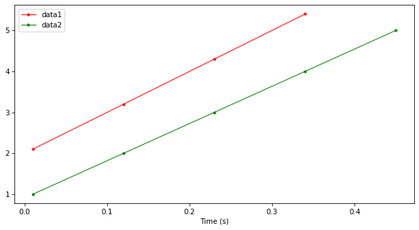
Using ktk.TimeSeries.resample, we can either resample instrument2 over instrument1’s time:

resampled_instrument2 = instrument2.resample(instrument1.time)

instrument1.plot("data1", "r.-")
resampled_instrument2.plot("data2", "g.-")

or resample instrument1 over instrument2’s time:

resampled_instrument1 = instrument1.resample(instrument2.time)

resampled_instrument1.plot("data1", "r.-")
instrument2.plot("data2", "g.-")

Tip

We already learned the ktk.TimeSeries.merge method to combine two TimeSeries. If both TimeSeries have different sampling rates as in the previous example, then ktk.TimeSeries.merge will fail. We need to resample the TimeSeries before merging them, as we did above.

ts1 = ts1.resample(ts2.time, kind="...")
ts1 = ts1.merge(ts1)

However, as a shortcut, ktk.TimeSeries.merge can also do the resampling for us using a linear interpolation:

ts1 = ts1.merge(ts2, resample=True)

7.2.3.3. Time shifting

In the original TimeSeries, we observe a brief transient in the signal that may be generated by an impact or pulse just before the action. It is common to generate such transients in data acquisition to synchronize data from different instruments. In this case, we may want to time-shift the TimeSeries so that this synchronization signal happens at 0 seconds. To do so, we use ktk.TimeSeries.shift:

synced_ts = ts.shift(-7.32)  # Subtract every time, including events, by 7.32

which gives: